BRIEF HISTORY OF GRATING DEVELOPMENT

A diffraction grating is a collection of reflecting (or transmitting) elements separated by a distance comparable to the wavelength of light under study. It may be thought of as a collection of diffracting elements, such as a pattern of transparent slits (or apertures) in an opaque screen, or a collection of reflecting grooves on a substrate. A reflection grating consists of a grating superimposed on a reflective surface, whereas a transmission grating consists of a grating superimposed on a transparent surface. An electromagnetic wave incident on a grating will, upon diffraction, have its electric field amplitude, or phase, or both, modified in a predictable manner.
The first diffraction grating was made by an American astronomer, David Rittenhouse, in 1785, who reported constructing a half-inch wide grating with fifty-three apertures. Apparently he developed this prototype no further, and there is no evidence that he tried to use it for serious scientific experiments. In 1821, unaware of the earlier American report, Joseph von Fraunhofer began his work on diffraction gratings. His research was given impetus by his insight into the value that grating dispersion could have for the new science of spectroscopy. Fraunhofer's persistence resulted in gratings of sufficient quality to enable him to measure the absorption lines of the solar spectrum. He also derived the equations that govern the dispersive behavior of gratings. Fraunhofer was interested only in making gratings for his own experiments, and upon his death, his equipment disappeared.
By 1850, F.A. Nobert, a Prussian instrument maker, began to supply scientists with gratings superior to Fraunhofer's. About 1870, the scene of grating development returned to America, where L.M. Rutherfurd, a New York lawyer with an avid interest in astronomy, became interested in gratings. In just a few years, Rutherfurd learned to rule reflection gratings in speculum metal that were far superior to any that Nobert had made. Rutherfurd developed gratings that surpassed even the most powerful prisms. He made very few gratings, though, and their uses were limited.
Rutherfurd's part-time dedication, impressive as it was, could not match the tremendous strides made by H.A. Rowland, professor of physics at the Johns Hopkins University. Rowland's work established the grating as the primary optical element of spectroscopic technology. Rowland constructed sophisticated ruling engines and invented the concave grating, a device of spectacular value to modern spectroscopists. He continued to rule gratings until his death in 1901.
After Rowland's great success, many people set out to rule diffraction gratings. The few who were successful sharpened the scientific demand for gratings. As the advantages of gratings over prisms and interferometers for spectroscopic work became more apparent, the demand for diffraction gratings far exceeded the supply. In 1947, Bausch & Lomb decided to make precision gratings available commercially. In 1950, through the encouragement of Prof. George R. Harrison of MIT, David Richardson and Robert Wiley of Bausch & Lomb succeeded in producing their first high quality grating. This was ruled on a rebuilt engine that had its origins in the University of Chicago laboratory of Prof. Albert A. Michelson. A high fidelity replication process was subsequently developed, which was crucial to making replicas, duplicates of the tediously generated master gratings. A most useful feature of modern gratings is the availability of an enormous range of sizes and groove spacings (up to 10,800 grooves per millimeter), and their enhanced quality is now almost taken for granted. In particular, the control of groove shape (or blazing) has increased spectral efficiency dramatically. In addition, interferometric and servo control systems have made it possible to break through the accuracy barrier previously set by the mechanical constraints inherent in the ruling engines.

THE GRATING EQUATION

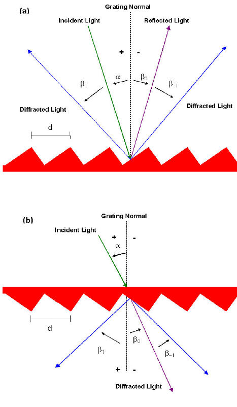
When monochromatic light is incident on a grating surface, it is diffracted into discrete directions. We can picture each grating groove as being a very small, slit-shaped source of diffracted light. The light diffracted by each groove combines to form a diffracted wavefront. The usefulness of a grating depends on the fact that there exists a unique set of discrete angles along which, for a given spacing d between grooves, the diffracted light from each facet is in phase with the light diffracted from any other facet, so they combine constructively. Diffraction by a grating can be visualized from the geometry in Figure 20, which shows a light ray of wavelength $\lambda$ incident at an angle $\alpha$ and diffracted by a grating (of groove spacing d, also called the pitch) along angles $\beta_m$ . These angles are measured from the grating normal, which is the dashed line perpendicular to the grating surface at its center. The sign convention for these angles depends on whether the light is diffracted on the same side or the opposite side of the grating as the incident light. In diagram (a), which shows a reflection grating, the angles $\alpha > 0$ and $\beta_1 > 0$ (since they are measured counter clockwise from the grating normal) while the angles $\beta_0 < 0$ and $\beta_-1 < 0$ (since they are measured clockwise from the grating normal). Diagram (b) shows the case for a transmission grating. By convention, angles of incidence and diffraction are measured from the grating normal to the beam.
This is shown by arrows in the diagrams. In both diagrams, the sign convention for angles is shown by the plus and minus symbols located on either side of the grating normal. For either reflection or transmission gratings, the algebraic signs of two angles differ if they are measured from opposite sides of the grating normal. Other sign conventions exist, so care must be taken in calculations to ensure that results are self-consistent. Another illustration of grating diffraction, using wave fronts (surfaces of constant phase), is shown in Figure 21.

Figure 20 - Diffraction by a plane grating. A beam of monochromatic light of wavelength is incident on a grating and diffracted along several discrete paths. The triangular grooves come out of the page; the rays lie in the plane of the page. The sign convention for the angles and is shown by the + and - signs on either side of the grating normal. (a) A reflection grating: the incident and diffracted rays lie on the same side of the grating. (b) A transmission grating: the incident and diffracted rays lies on opposite sides of the grating.

The geometrical path difference between light from adjacent grooves is seen to be [Since $\beta$ < 0, the latter term is actually negative.] The principle of interference dictates that only when this difference equals the wavelength $\lambda$ of the light, or some integral multiple thereof, will the light from adjacent grooves be in phase (leading to constructive interference). At all other angles $\beta$ , there will be some measure of destructive interference between the wavelets originating from the groove facets.
These relationships are expressed by the grating equation:

$m\lambda=(\sin\alpha + \sin\beta) \qquad \qquad \qquad (1)$

which governs the angles of diffraction from a grating of groove spacing d. Here m is the diffraction order (or spectral order), which is an integer. For a particular wavelength , all values of m for which |m /d| < 2 correspond to physically realizable diffraction orders.
It is sometimes convenient to write the grating equation as:

$Gm=(\sin\alpha + \sin\beta) \qquad \qquad \qquad (2)$

where G = 1/d is the groove frequency or groove density, more commonly called "grooves per millimeter". Eq. (1) and its equivalent Eq. (2) are the common forms of the grating equation, but their validity is restricted to cases in which the incident and diffracted rays are perpendicular to the grooves (at the center of the grating). The vast majority of grating systems fall within this category, which is called classical (or in-plane) diffraction. If the incident light beam is not perpendicular to the grooves, though, the grating equation must be modified:

$Gm\lambda= \cos\epsilon(\sin\alpha + \sin\beta) \qquad \qquad \qquad (3)$

Here $\epsilon$ is the angle between the incident light path and the plane perpendicular to the grooves at the grating center (the plane of the page in Figure 4.21). If the incident light lies in this plane, $\epsilon$ = 0 and Eq. (3) reduces to the more familiar Eq. (2). In geometries for which $\epsilon$ = 0, the diffracted spectra lie on a cone rather than in a plane, so such cases are termed conical diffraction.
For a grating of groove spacing d, there is a purely mathematical relationship between the wavelength and the angles of incidence and diffraction. In a given spectral order m, the different wavelengths of polychromatic wavefronts incident at angle $\alpha$ are separated in angle:

$\beta \left( \lambda \right) =\arcsin (\frac{m\lambda }{d}-\sin\alpha ) \qquad \qquad \qquad (4)$

When m = 0, the grating acts as a mirror, and the wavelengths are not separated ( $\beta = -\alpha$ , for all $\lambda$ ); this is called specular reflection or simply the zero order.

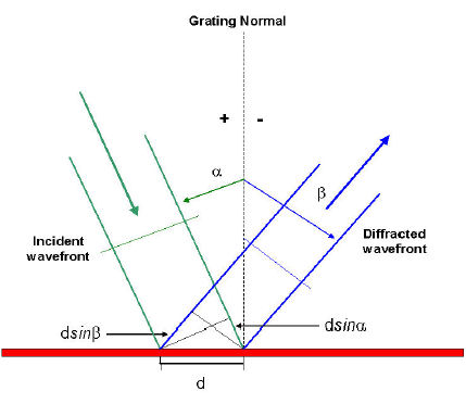
Figure 21 - Geometry of diffraction for planar wavefront.
The terms in the path difference, $d\sin\alpha$ and $d\sin\beta$ , are shown A special but common case is that in which the light is diffracted back toward the direction from which it came (i.e., $\alpha = \beta$ ); this is called the Littrow configuration, for which the grating equation becomes:

$m\lambda = 2d\sin\alpha, \qquad in Littrow \qquad (5)$

. In many applications (such as constant-deviation monochromators), the wavelength $\alpha$ is changed by rotating the grating about the axis coincident with its central ruling, with the directions of incident and diffracted light remaining unchanged. The deviation angle 2K between the incidence and diffraction directions (also called the angular deviation) is

$2K = \alpha - \beta = constant \qquad \qquad \qquad (6)$

while the scan angle $\phi$ , which is measured from the grating normal to the bisector of the beams, is

$2\phi = \alpha + \beta \qquad \qquad \qquad (7)$

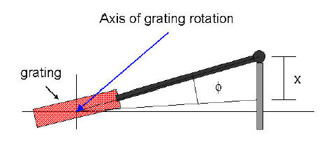
Figure 22 - A sine bar mechanism for wavelength scanning.
As the screw is extended linearly by the distance x shown, the grating rotates through an angle $\phi$ in such a way that $\sin\phi$ is proportional to x Note that $\phi$ changes with $\lambda$ (as do $\alpha$ and $\beta$ ). In this case, the grating equation can be expressed in terms of $\phi$ and the half deviation angle K as:

$m\lambda = 2d\cos K\sin\phi \qquad \qquad \qquad (8)$

This version of the grating equation is useful for monochromator mounts.
Eq. (8) shows that the wavelength diffracted by a grating in a monochromator mount is directly proportional to the sine of the angle $\phi$ through which the grating rotates, which is the basis for monochromator drives in which a sine bar rotates the grating to scan wavelengths (see Figure 22).

DIFFRACTION ORDERS

Existence of Diffraction Orders

For a particular set of values of the groove spacing d and the angles $\alpha$ and $\beta$ , the grating equation (1) is satisfied by more than one wavelength. In fact, subject to restrictions discussed below, there may be several discrete wavelengths which, when multiplied by successive integers m, satisfy the condition for constructive interference. The physical significance of this is that the constructive reinforcement of wavelets diffracted by successive grooves merely requires that each ray be retarded (or advanced) in phase with every other; this phase difference must therefore correspond to a real distance (path difference) which equals an integral multiple of the wavelength. This happens, for example, when the path difference is one wavelength, in which case we speak of the positive first diffraction order (m = 1) or the negative first diffraction order (m = -1), depending on whether the rays are advanced or retarded as we move from groove to groove. Similarly, the second order (m = 2) and negative second order (m = -2) are those for which the path difference between rays diffracted from adjacent grooves equals two wavelengths.
The grating equation reveals that only those spectral orders for which $|m\lambda /d| < 2$ can exist; otherwise, $|\sin\alpha + \sin\beta| > 2$ , which is physically meaningless. This restriction prevents light of wavelength $\lambda$ from being diffracted in more than a finite number of orders. Specular reflection (m = 0) is always possible; that is, the zero order always exists (it simply requires $\alpha = -\beta$ ). In most cases, the grating equation allows light of wavelength $\lambda$ to be diffracted into both negative and positive orders as well. Explicitly, spectra of all orders m exist for which

$-2d < m\lambda < 2d, m an integer. \qquad \qquad \qquad (9)$

For l/d << 1, a large number of diffracted orders will exist. As seen from Eq. (1), the distinction between negative and positive spectral orders is that

$\beta > -\alpha \qquad for positive orders (m > 0),$

$\beta < -\alpha \qquad for negative orders (m < 0),\qquad \qquad \qquad (9')$

$\beta = -\alpha \qquad for specular reflection (m = 0),$

This sign convention for m requires that m > 0 if the diffracted ray lies to the left (the counter-clockwise side) of the zero order (m = 0), and m < 0 if the diffracted ray lies to the right (the clockwise side) of the zero order. This convention is shown graphically in Figure 23.

Overlapping of Diffracted Spectra

The most troublesome aspect of multiple order behavior is that successive spectra overlap, as shown in Figure 24. It is evident from the grating equation that, for any grating instrument configuration, the light of wavelength $\lambda$ diffracted in the m = 1 order will coincide with the light of wavelength $\lambda/2$ diffracted in the m = 2 order, etc., for all m satisfying inequality (9). In this example, the red light (600 nm) in the first spectral order will overlap the ultraviolet light (300 nm) in the second order. A detector sensitive at both wavelengths would see both simultaneously. This superposition of wavelengths, which would lead to ambiguous spectroscopic data, is inherent in the grating equation itself and must be prevented by suitable filtering (called order sorting), since the detector cannot generally distinguish between light of different wavelengths incident on it (within its range of sensitivity).

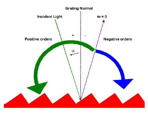
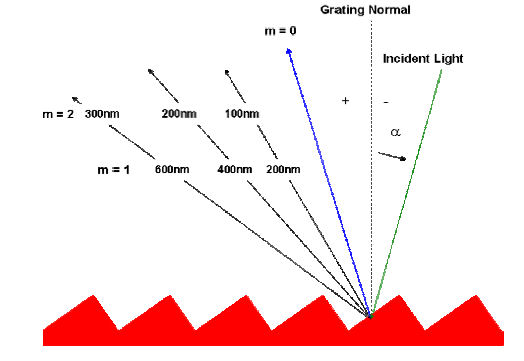
Figure 23 - Sign convention for the spectral order m. In this example is positive.

Figure 24 - Overlapping of spectral orders. The light for wavelengths 100, 200 and 300 nm in the second order is diffracted in the same direction as the light for wavelengths 200, 400 and 600 nm in the first order. In this diagram, the light is incident from the right, so $\alpha < 0$ .

DISPERSION

The primary purpose of a diffraction grating is to disperse light spatially by wavelength. A beam of white light incident on a grating will be separated into its component colors upon diffraction from the grating, with each color diffracted along a different direction. Dispersion is a measure of the separation (either angular or spatial) between diffracted light of different wavelengths. Angular dispersion expresses the spectral range per unit angle, and linear resolution expresses the spectral range per unit length.

Angular dispersion

The angular spread $d\beta$ of a spectrum of order m between the wavelength $\lambda$ and $\lambda + d\lambda$ can be obtained by differentiating the grating equation, assuming the incidence angle $\alpha$ to be constant. The change D in diffraction angle per unit wavelength is therefore:

$D=\frac{\partial \beta }{\partial \lambda }=\frac{m}{d\cos \beta }=\frac{m}{d}\sec \beta =Gm\sec \beta \qquad \qquad (10)$

where is given by Eq. (2-2). The ratio D = d /d is called the angular dispersion. As the groove frequency G = 1/d increases, the angular dispersion increases (meaning that the angular separation between wavelengths increases for a given order m). In Eq. (2-9), it is important to realize that the quantity m/d is not a ratio which may be chosen independently of other parameters; substitution of the grating equation into Eq. (2-9) yields the following general equation for the angular dispersion: (2-10) For a given wavelength, this shows that the angular dispersion may be considered to be solely a function of the angles of incidence and diffraction. This becomes even more clear when we consider the Littrow configuration ( = ), in which case Eq. (2-10) reduces to , in Littrow. (2-11)

When | | increases from 10� to 63� in Littrow use, the angular dispersion increases by a factor of ten, regardless of the spectral order or wavelength under consideration. Once has been determined, the choice must be made whether a fine-pitch grating (small d) should be used in a low order, or a course-pitch grating (large d) such as an echelle grating should be used in a high order. [The fine-pitched grating, though, will provide a larger free spectral range; see Section 2.7 below.]

Linear dispersion

For a given diffracted wavelength in order m (which corresponds to an angle of diffraction ), the linear dispersion of a grating system is the product of the angular dispersion D and the effective focal length r' ( ) of the system: (2-12) The quantity r' d = dl is the change in position along the spectrum (a real distance, rather than a wavelength). We have written r' ( ) for the focal length to show explicitly that it may depend on the diffraction angle (which, in turn, depends on ). The reciprocal linear dispersion, also called the plate factor P, is more often considered; it is simply the reciprocal of r' D, usually measured in nm/mm: (2-12') P is a measure of the change in wavelength (in nm) corresponding to a change in location along the spectrum (in mm). It should be noted that the terminology plate factor is used by some authors to represent the quantity 1/sin , where is the angle the spectrum makes with the line perpendicular to the diffracted rays (see Figure 2-6); in order to avoid confusion, we call the quantity 1/sin the obliquity factor. When the image plane for a particular wavelength is not perpendicular to the diffracted rays (i.e., when 90�), P must be multiplied by the obliquity factor to obtain the correct reciprocal linear dispersion in the image plane.

The obliquity angle . The spectral image recorded need not lie in the plane perpendicular to the diffracted ray (i.e., ? 90�)

Resolving power

The resolving power R of a grating is a measure of its ability to separate adjacent spectral lines of average wavelength . It is usually expressed as the dimensionless quantity (2-13) Here is the limit of resolution, the difference in wavelength between two lines of equal intensity that can be distinguished (that is, the peaks of two wavelengths and 2 for which the separation | 1 - 2| < will be ambiguous). The theoretical resolving power of a planar diffraction grating is given in elementary optics textbooks as (2-14) where m is the diffraction order and N is the total number of grooves illuminated on the surface of the grating. For negative orders (m < 0), the absolute value of R is considered. A more meaningful expression for R is derived below. The grating equation can be used to replace m in Eq. (2-14): (2-15) If the groove spacing d is uniform over the surface of the grating, and if the grating substrate is planar, the quantity Nd is simply the ruled width W of the grating, so (2-16) As expressed by Eq. (2-16), R is not dependent explicitly on the spectral order or the number of grooves; these parameters are contained within the ruled width and the angles of incidence and diffraction. Since (2-17) the maximum attainable resolving power is (2-18) regardless of the order m or number of grooves N. This maximum condition corresponds to the grazing Littrow configuration, i.e., (Littrow), (grazing). It is useful to consider the resolving power as being determined by the maximum phase retardation of the extreme rays diffracted from the grating. Measuring the difference in optical path lengths between the rays diffracted from opposite sides of the grating provides the maximum phase retardation; dividing this quantity by the wavelength of the diffracted light gives the resolving power R. The degree to which the theoretical resolving power is attained depends not only on the angles and , but also on the optical quality of the grating surface, the uniformity of the groove spacing, the quality of the associated optics, and the width of the slits and/or detector elements. Any departure of the diffracted wavefront greater than /10 from a plane (for a plane grating) or from a sphere (for a spherical grating) will result in a loss of resolving power due to aberrations at the image plane. The grating groove spacing must be kept constant to within about 1% of the wavelength at which theoretical performance is desired. Experimental details, such as slit width, air currents, and vibrations can seriously interfere with obtaining optimal results. The practical resolving power is limited by the spectral half-width of the lines emitted by the source. This explains why systems with revolving powers greater than 500,000 are usually required only in the study of spectral line shapes, Zeeman effects, and line shifts, and are not needed for separating individual spectral lines. A convenient test of resolving power is to examine the isotopic structure of the mercury emission line at 546.1 nm. Another test for resolving power is to examine the line profile generated in a spectrograph or scanning spectrometer when a single mode laser is used as the light source. Line width at half intensity (or other fractions as well) can be used as the criterion. Unfortunately, resolving power measurements are the convoluted result of all optical elements in the system, including the locations and dimensions of the entrance and exit slits and the auxiliary lenses and mirrors, as well as the quality of these optics. Their effects are necessarily superimposed on those of the grating.

Spectral resolution

While resolving power can be considered a characteristic of the grating and the angles at which it is used, the ability to resolve two wavelengths 1 and 2 = 1 + generally depends not only on the grating but on the dimensions and locations of the entrance and exit slits (or detector elements), the aberrations in the images, and the magnification of the images. The minimum wavelength difference (also called the limit of resolution, or simply resolution) between two wavelengths that can be resolved unambiguously can be determined by convoluting the image of the entrance aperture (at the image plane) with the exit aperture (or detector element). This measure of the ability of a grating system to resolve nearby wavelengths is arguably more relevant than is resolving power, since it takes into account the image effects of the system. While resolving power is a dimensionless quantity, resolution has spectral units (usually nanometers).

Bandpass

The bandpass B of a spectroscopic system is the wavelength interval of the light that passes through the exit slit (or falls onto a detector element). It is often defined as the difference in wavelengths between the points of half-maximum intensity on either side of an intensity maximum. An estimate for bandpass is the product of the exit slit width w' and the reciprocal linear dispersion P: ..(2-19) An instrument with smaller bandpass can resolve wavelengths that are closer together than an instrument with a larger bandpass. Bandpass can be reduced by decreasing the width of the exit slit (to a certain limit; see Chapter 8), but usually at the expense of decreasing light intensity as well. Bandpass is sometimes called spectral bandwidth, though some authors assign distinct meanings to these terms. Resolving power vs. resolution
In the literature, the terms resolving power and resolution are sometimes interchanged. While the word power has a very specific meaning (energy per unit time), the phrase resolving power does not involve power in this way; as suggested by Hutley, though, we may think of resolving power as 'ability to resolve'. The comments above regarding resolving power and resolution pertain to planar classical gratings used in collimated light (plane waves). The situation is complicated for gratings on concave substrates or with groove patterns consisting of unequally spaced lines, which restrict the usefulness of the previously defined simple formulae, though they may still yield useful approximations. Even in these cases, though, the concept of maximum retardation is still a useful measure of the resolving power.

FOCAL LENGTH AND f/NUMBER

For gratings (or grating systems) that image as well as diffract light, or disperse light that is not collimated, a focal length may be defined. If the beam diffracted from a grating of a given wavelength and order m converges to a focus, then the distance between this focus and the grating center is the focal length r'( ). [If the diffracted light is collimated, and then focused by a mirror or lens, the focal length is that of the refocusing mirror or lens and not the distance to the grating.] If the diffracted light is diverging, the focal length may still be defined, although by convention we take it to be negative (indicating that there is a virtual image behind the grating). Similarly, the incident light may diverge toward the grating (so we define the incidence or entrance slit distance r( ) > 0) or it may converge toward a focus behind the grating (for which r( ) < 0). Usually gratings are used in configurations for which r does not depend on wavelength (though in such cases r' usually depends on ). In Figure 2-7, a typical concave grating configuration is shown; the monochromatic incident light (of wavelength ) diverges from a point source at A and is diffracted toward B. Points A and B are distances r and r', respectively, from the grating center O. In this figure, both r and r' are positive. Calling the width (or diameter) of the grating (in the dispersion plane) W allows the input and output �/numbers (also called focal ratios) to be defined: (2-20) Usually the input �/number is matched to the �/number of the light cone leaving the entrance optics (e.g., an entrance slit or fiber) in order to use as much of the grating surface for diffraction as possible. This increases the amount of diffracted energy while not overfilling the grating (which would generally contribute to stray light). For oblique incidence or diffraction, Eqs. (2-20) are often modified by replacing W with the projected width of the grating: (2-21) These equations account for the reduced width of the grating as seen by the entrance and exit slits; moving toward oblique angles (i.e., increasing | | or | |) decreases the projected width and therefore increases the �/number. Figure 2-7. Geometry for focal distances and focal ratios (�/numbers). GN is the grating normal (perpendicular to the grating at its center, O), W is the width of the grating (its dimension perpendicular to the groove direction, which is out of the page), and A and B are the source and image points, respectively. Figure 4.26 The focal length is an important parameter in the design and specification of grating spectrometers, since it governs the overall size of the optical system (unless folding mirrors are used). The ratio between the input and output focal lengths determines the projected width of the entrance slit that must be matched to the exit slit width or detector element size. The �/number is also important, as it is generally true that spectral aberrations decrease as �/number increases. Unfortunately, increasing the input �/number results in the grating subtending a smaller solid angle as seen from the entrance slit; this will reduce the amount of light energy the grating collects and consequently reduce the intensity of the diffracted beams. This trade-off prohibits the formulation of a simple rule for choosing the input and output �/numbers, so sophisticated design procedures have been developed to minimize aberrations while maximizing collected energy. See Chapter 7 for a discussion of the imaging properties and Chapter 8 for a description of the efficiency characteristics of grating systems.

ANAMORPHIC MAGNIFICATION

For a given wavelength , we may consider the ratio of the width of a collimated diffracted beam to that of a collimated incident beam to be a measure of the effective magnification of the grating (see Figure 2-8). From this figure we see that this ratio is (2-22) Since and depend on through the grating equation (2-1), this magnification will vary with wavelength. The ratio b/a is called the anamorphic magnification; for a given wavelength , it depends only on the angular configuration in which the grating is used. Figure 2-8. Anamorphic magnification. The ratio b/a of the beam widths equals the anamorphic magnification. Figure 4.27 The magnification of an object not located at infinity (so that the incident rays are not collimated) is discussed in Chapter 8.

FREE SPECTRAL RANGE

For a given set of incidence and diffraction angles, the grating equation is satisfied for a different wavelength for each integral diffraction order m. Thus light of several wavelengths (each in a different order) will be diffracted along the same direction: light of wavelength in order m is diffracted along the same direction as light of wavelength /2 in order 2m, etc. The range of wavelengths in a given spectral order for which superposition of light from adjacent orders does not occur is called the free spectral range F . It can be calculated directly from its definition: in order m, the wavelength of light that diffracts along the direction of 1 in order m+1 is where: (2-23) from which (2-24) The concept of free spectral range applies to all gratings capable of operation in more than one diffraction order, but it is particularly important in the case of echelles, because they operate in high orders with correspondingly short free spectral ranges. Free spectral range and order sorting are intimately related, since grating systems with greater free spectral ranges may have less need for filters (or cross-dispersers) that absorb or diffract light from overlapping spectral orders. This is one reason why first-order applications are widely popular.

ENERGY DISTRIBUTION (GRATING EFFICIENCY)

The distribution of incident field power of a given wavelength diffracted by a grating into the various spectral order depends on many parameters, including the power and polarization of the incident light, the angles of incidence and diffraction, the (complex) index of refraction of the metal (or glass or dielectric) of the grating, and the groove spacing. A complete treatment of grating efficiency requires the vector formalism of electromagnetic theory (i.e., Maxwell's equations), which has been studied in detail over the past few decades. While the theory does not yield conclusions easily, certain rules of thumb can be useful in making approximate predictions. Recently, computer codes have become commercially available that accurately predict grating efficiency for a wide variety of groove profiles over wide spectral ranges.

SCATTERED AND STRAY LIGHT

All light that reaches the image plane from anywhere other than the grating, by any means other than diffraction as governed by Eq. (2-1), is called stray light. All components in an optical system contribute stray light, as will any baffles, apertures, and partially reflecting surfaces. Unwanted light originating from the grating itself is often called scattered light.

Scattered light

Of the radiation incident on the surface of a diffraction grating, some will be diffracted according to Eq. (2-1) and some will be absorbed by the grating itself. The remainder is unwanted energy called scattered light. Scattered light may arise from several factors, including imperfections in the shape and spacing of the grooves and roughness on the surface of the grating. Diffuse scattered light is scattered into the hemisphere in front of the grating surface. It is due mainly to grating surface microroughness. It is the primary cause of scattered light in interference gratings. For monochromatic light incident on a grating, the intensity of diffuse scattered light is higher near the diffraction orders for that wavelength than between the diffracted orders. M.C. Hutley (National Physical Laboratory) found this intensity to be proportional to slit area, and probably proportional to 1/ . In-plane scatter is unwanted energy in the dispersion plane. Due primarily to random variations in the groove spacing or groove depth, its intensity is directly proportional to slit area and probably inversely proportional to the square of the wavelength. Ghosts are caused by periodic errors in the groove spacing. Characteristic of ruled gratings, interference gratings are free from ghosts when properly made.

Instrumental stray light

Stray light for which the grating cannot be blamed is called instrumental stray light. Most important is the ever-present light reflected into the zero order, which must be trapped so that it does not contribute to stray light. Light diffracted into other orders may also find its way to the detector and therefore constitute stray light. Diffraction from sharp edges and apertures causes light to propagate along directions other than those predicted by the grating equation. Reflection from instrument chamber walls and mounting hardware also contributes to the redirection of unwanted energy toward the image plane; generally, a smaller instrument chamber presents more significant stray light problems. Light incident on detector elements may be reflected back toward the grating and rediffracted; since the angle of incidence may now be different, light rediffracted along a given direction will generally be of a different wavelength than the light that originally diffracted along the same direction. Baffles, which trap diffracted energy outside the spectrum of interest, are intended to reduce the amount of light in other orders and in other wavelengths, but they may themselves diffract and reflect this light so that it ultimately reaches the image plane.

SIGNAL-TO-NOISE RATIO (SNR)

The signal-to-noise ratio (SNR) is the ratio of diffracted energy to unwanted light energy. While we might be tempted to think that increasing diffraction efficiency will increase SNR, stray light usually plays the limiting role in the achievable SNR for a grating system. Replicated gratings from ruled master gratings generally have quite high SNRs, though holographic gratings sometimes have even higher SNRs, since they have no ghosts due to periodic errors in groove location and lower interorder stray light. As SNR is an instrument function, not a property of the grating only, there exist no clear rules of thumb regarding what type of grating will provide higher SNR.

CLASSICAL CONCAVE GRATING IMAGING

A concave reflection grating can be modeled as a concave mirror that disperses; it can be thought to reflect and focus light by virtue of its concavity, and to disperse light by virtue of its groove pattern. Since their invention by Henry Rowland in 1883, concave diffraction gratings have played an important role in spectrometry. Compared with plane gratings, they offer one important advantage: they provide the focusing (imaging) properties to the grating that otherwise must be supplied by separate optical elements. For spectroscopy below 110 nm, for which the reflectivity of available mirror coatings is low, concave gratings allow for systems free from focusing mirrors that would reduce throughput two or more orders of magnitude. Many configurations for concave spectrometers have been proposed. Some are variations of the Rowland circle, while some place the spectrum on a flat field, which is more suitable for charge-coupled device (CCD) array instruments. The Seya-Namioka concave grating monochromator is especially suited for scanning the spectrum by rotating the grating around its own axis. In Figure 7-1, a classical grating is shown; the Cartesian axes are defined as follows: the x-axis is the outward grating normal to the grating surface at its center (point O), the y-axis is tangent to the grating surface at O and perpendicular to the grooves there, and the z-axis completes the right-handed triad of axes (and is therefore parallel to the grooves at O). Light from point source A( , , 0) is incident on a grating at point O; light of wavelength in order m is diffracted toward point B( ', ', 0). Since point A was assumed, for simplicity, to lie in the xy plane, to which the grooves are perpendicular at point O, the image point B will lie in this plane as well; this plane is called the principal plane (also called the tangential plane or the dispersion plane (see Figure 7-2). Ideally, any point P(x, y, z) located on the grating surface will also diffract light from A to B. The plane through points O and B perpendicular to the principal plane is called the sagittal plane, which is unique for this wavelength. The grating tangent plane is the plane tangent to the grating surface at its center point O (i.e., the yz plane). The imaging effects of the groove spacing and curvature can be completely separated from those due to the curvature of the substrate if the groove pattern is projected onto this plane. Figure 7-1. Use geometry. The grating surface centered at O diffracts light from point A to point B. P is a general point on the grating surface. The x-axis points out of the grating from its center, the z-axis points along the central groove, and the y-axis completes the traid. Figure 4.28 The imaging of this optical system can be investigated by considering the optical path difference OPD between the pole ray AOB (where O is the center of the grating) and the general ray APB (where P is an arbitrary point on the grating surface). Application of Fermat's principle to this path difference, and the subsequent expansion of the results in power series of the coordinates of the tangent plane (y and z), yields expressions for the aberrations of the system. Figure 7-2. Use geometry - the principal plane. Points A, B and O lie in the xy (principal) plane; the general point P on the grating surface may lie outside this plane. The z-axis comes out of the page at O. Figure 4.29

The optical path difference is:

(7-1)

where (APB) and (AOB) are the geometric lengths of the general and pole rays, respectively (both multiplied by the index of refraction), m is the diffraction order, and N is the number of grooves on the grating surface between points O and P. The last term in Eq. (7-1) accounts for the fact that the distances and need not be exactly equal for the light along both rays to be in phase at B: due to the wave nature of light, the light is in phase at B even if there are an integral number of wavelengths between these two distances. If points O and P are one groove apart (N = 1), the number of wavelengths in the difference determines the order of diffraction m. From geometric considerations, we find

(7-2)

and similarly for (AOB), if the medium of propagation is air ( ). The optical path difference can be expressed more simply if the coordinates of points A and B are plane polar rather than Cartesian: letting (AO) = r, (OB) = r', (7-3) we may write = r cos , = r sin ; (7-4) ' = r' cos , ' = r' sin ;

where the angles of incidence and diffraction ( and ) follow the sign convention described in Chapter 2. The power series for OPD can be written in terms of the grating surface point coordinates y and z:

, (7-5)

where Fij, the expansion coefficient of the (i,j) term, describes how the rays (or wavefronts) diffracted from point P toward the ideal image point B differ (in direction, or curvature, etc.) in proportion to yiz from those from point O. The x-dependence of OPD has been suppressed by writing

, (7-6)

This equation makes use of the fact that the grating surface is usually a regular function of position, so x is not independent of y and z (i.e., if it is a spherical surface of radius R, then By analogy with the terminology of lens and mirror optics, we call each term in series (7-5) an aberration, and Fij its aberration coefficient. An aberration is absent from the image of a given wavelength (in a given diffraction order) if its associated coefficient Fij is zero. Since we have imposed a plane of symmetry on the system (the principal (xy) plane), all terms Fij for which j is odd vanish. Moreover, F00 = 0, since the expansion (7-5) is about the origin O. The lowest- (first-) order term F10 in the expansion, when set equal to zero, yields the grating equation:

m = d (sin + sin ). (2-1)

By Fermat's principle, we may take this equation to be satisfied for all images, which leaves the second-order aberration terms as those of lowest order that need not vanish. The generally accepted terminology is that a stigmatic image has vanishing second-order coefficients even if higher-order aberrations are still present.

 (7-7)

 (7-8)

F20 governs the tangential (or spectral) focusing of the grating system, while F02 governs the sagittal focusing. The associated aberrations are called defocus and astigmatism, respectively. The two aberrations describe the extent of a monochromatic image: defocus pertains to the blurring of the image - its extent of the image along the dispersion direction (i.e., in the tangential plane). Astigmatism pertains to the extent of the image in the direction perpendicular to the dispersion direction. In more common (but sometimes misleading) terminology, defocus applies to the "width" of the image in the spectral (dispersion) direction, and astigmatism applies to the "height" of the spectral image; these terms imply that the xy (tangential) plane be considered as "horizontal" and the yz (sagittal) plane as "vertical". Actually astigmatism more correctly defines the condition in which the tangential and sagittal foci are not coincident, which implies a line image at the tangential focus. It is a general result of the off-axis use of a concave mirror (and, by extension, a concave reflection grating as well). A complete three-dimensional treatment of OPD shows that the image is actually an arc; image points away from the center of the ideal image are diffracted toward the longer wavelengths. This effect, which technically is not an aberration, is called (spectral) line curvature, and is most noticeable in the spectra of Paschen-Runge mounts (see later in this chapter). Figure 7-3 shows astigmatism in the image of a wavelength diffracted off-axis from a concave grating, ignoring line curvature. Since grating images are generally astigmatic, the focal distances r' in Eqs. (7-7) and (7-8) should be distinguished. Calling r'T and r'S the tangential and sagittal focal distances, respectively, we may set these equations equal to zero and solve for the focal curves r'T( ) and r'S( ):

Figure 7-3. Astigmatic focusing of a concave grating. Light from point A is focused into a line parallel to the grooves at TF (the tangential focus) and perpendicular to the grooves at SF (the sagittal focus). Spectral resolution is maximized at TF.

Figure 4.30

(7-9)

(7-10)

Here we have defined

(7-11)

where a20 and a02 are the coefficients in Eq. (7-6) (e.g., a20 = a02 = 1/(2R) for a spherical grating of radius R). These expressions are completely general for classical grating systems; that is, they apply to any type of grating mount or configuration. Of the two primary (second-order) focal curves, that corresponding to defocus (F20) is of greater importance in spectroscopy, since it is spectral resolution that is most crucial to grating systems. For this reason we do not concern ourselves with locating the image plane at the "circle of least confusion"; rather, we try to place the image plane at or near the tangential focus (where F20 = 0). For concave gratings ( ) there are two well-known solutions to the defocus equation F20 = 0. The Rowland circle is a circle whose diameter is equal to the tangential radius of the grating substrate, and which passes through the grating center (point O in Figure 7-5). If the point source A is placed on this circle, the tangential focal curve also lies on this circle. This solution is the basis for the Rowland circle and Paschen-Runge mounts. For the Rowland circle mount,

(7-12)

The sagittal focal curve is

 (7-13)

(where is the sagittal radius of the grating), which is always greater than r'T (even for a spherical substrate, for which = R) unless = = 0. Consequently this mount suffers from astigmatism, which in some cases is considerable. The Wadsworth mount is one in which the source light is collimated ( ), so that the tangential focal curve is given by

(7-14)

The sagittal focal curve is

(7-15)

In this mount, the imaging from a classical spherical grating ( = R) is such that the astigmatism of the image is zero only for = 0, though this is true for any incidence angle . While higher-order aberrations are usually of less importance than defocus and astigmatism, they can be significant. T he third-order aberrations, primary or tangential coma F30 and secondary or sagittal coma F12, are given by

(7-15)

(7-16)

where T and S are defined in Eqs. (7-7) and (7-8). Often one or both of these third-order aberrations is significant in a spectral image, and must be minimized with the second-order aberrations.

The Rowland Circle Spectrograph

The first concave gratings of spectroscopic quality were ruled by Rowland, who invented them in 1881, also designing their first mounting. Placing the ideal source point on the Rowland circle forms spectra on that circle free from defocus and primary coma at all wavelengths (i.e., F20 = F30 = 0 for all ); while spherical aberration is residual and small, astigmatism is usually severe. Originally a Rowland circle spectrograph employed a photographic plate bent along a circular arc on the Rowland circle to record the spectrum in its entirety.

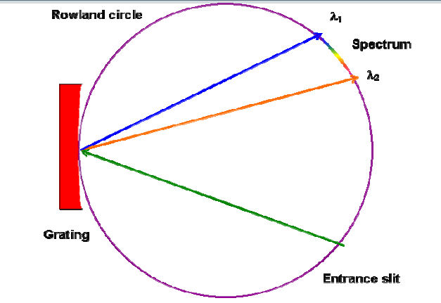
The Rowland Circle spectrograph. Both the entrance slit and the diffracted spectrum

lie on the Rowland circle, whose diameter equals the tangential radius of curvature R of the grating and that passes through the grating center. Light of two wavelengths is shown focused at different points on the Rowland circle."

Today it is more common for a series of exit slits to be cut into a circular mask to allow the recording of several discrete wavelengths photoelectrically; this system is called the Paschen-Runge mount. Other configurations based on the imaging properties of the Rowland circle are the Eagle mount and the Abney mount, both of which are described by Hutley and by Meltzer (see the Bibliography). Unless the exit slits (or photographic plates) are considerably taller than the entrance slit, the astigmatism of Rowland circle mounts usually prevents more than a small fraction of the diffracted light from being recorded, which greatly decreases the efficiency of the instrument. Increasing the exit slit heights helps collect more light, but since the images are curved, the exits slits would have to be curved as well to maintain optimal resolution. To complicate matters further, this curvature depends on the diffracted wavelength, so each exit slit would require a unique curvature. Few instruments have gone to such trouble, so most Rowland circle grating mounts collect only a small portion of the light incident on the grating. For this reason these mounts are adequate for strong sources (such as the observation of the solar spectrum) but not for less intense sources (such as stellar spectra). The imaging properties of instruments based on the Rowland circle spectrograph, such as direct readers and atomic absorption instruments, can be improved by the use of nonclassical gratings. Replacing the usual concave classical gratings with concave aberration-reduced gratings, astigmatism can be improved substantially. Rowland circle mounts modified in this manner direct more diffracted light through the exit slits without degrading resolution.

The Wadsworth Spectrograph

When a classical concave grating is illuminated with collimated light (rather than from a point source on the Rowland circle), spectral astigmatism on and near the grating normal is greatly reduced. Such a grating system is called the Wadsworth mount (see Figure 7-6). The wavelength-dependent aberrations of the grating are compounded by the aberration of the collimating optics, though use of a paraboloidal mirror illuminated on-axis will eliminate off-axis aberrations and spherical aberrations. The Wadsworth mount suggests itself in situations in which the light incident on the grating is naturally collimated (from, for example, synchrotron radiation sources). In other cases, an off-axis parabolic mirror would serve well as the collimating element. Figure 4.32

Constant-Deviation Monochromators

In a constant-deviation monochromator, the angle 2K between the entrance and exit arms is held constant as the grating is rotated (thus scanning the spectrum; see Figure 7-9). This angle is called the deviation angle or angular deviation. While plane or concave gratings can be used in constant-deviation mounts, only in the latter case can imaging be made acceptable over an entire spectrum without auxiliary focusing optics. Figure 4.33 The Seya-Namioka monochromator is a very special case of constant-deviation mount using a classical spherical grating, in which the deviation angle 2K between the beams and the entrance and exit slit distances (r and r') are given by 2K = 70�30', r = r' = R cos(70�30'/2), (7-24) where R is the radius of the spherical grating substrate. The only moving part in this system is the grating, through whose rotation the spectrum is scanned. Resolution may be quite good in part of the spectrum, though it degrades farther from the optimal wavelength; astigmatism is high, but at an optimum. Replacing the grating with a classical toroidal grating can reduce the astigmatism, if the minor radius of the toroid is chosen judiciously. The reduction of astigmatism by suitably designed interference gratings is also helpful, though the best way to optimize the imaging of a constant-deviation monochromator is to relax the restrictions (7-24) on the use geometry.